JRockit: How to Estimate the Size of Live Data Set

In [1], we have described our benchmark as having:

• Large Live Data Set

For instance, we have estimated that its live data size is approximately 1437MB using genconpar strategy.^[4] In this article, we will show how to estimate the size of live data set using another strategy genpar. As you can guess, the live data size of a benchmark could be different using different GC strategies. Basically, live data size depends on:

• Frequency of Objects Promoted from Young Gen (or Nursery) to Old Gen
• Frequency of Collections

which, in turn, depend on which GC strategy used.

Importance of Estimating Live Data Size

The mark-and-sweep algorithm is the basis of all commercial garbage collectors in JVMs (including JRockit) today.^[2,3] Here is how it works:^[2]

When the system starts running out of memory (or some other such trigger) the GC is fired. It first enumerates all the roots and then starts visiting the objects referenced by them recursively (essentially travelling the nodes in the memory graph). When it reaches an object it marks it with a special flag indicating that the object is reachable and hence not garbage. At the end of this mark phase it gets into the sweep phase. Any object in memory that is not marked by this time is garbage and the system disposes it.

As can be inferred from the above algorithm, the computational complexity of mark and sweep is both a function of the amount of live data on the heap (for mark) and the actual heap size (for sweep). If your application has a large live data set, it could be a garbage collection bottleneck. Any garbage collection algorithm could break down given too large an amount of live data. So, it's important to estimate the size of live data set in your Java applications for any performance evaluation.

How to Estimate the Live Data Size

To estimate the live data size, we have used:

• -Xverbose:gc flag

The format of the output is as follows:

<start>-<end>: <type> <before>KB-><after>KB (<heap>KB), <time> ms, sum of pauses <pause> ms.
<start> - start time of collection (seconds since jvm start).
<type> - OC (old collection) or YC (young collection).
<end> - end time of collection (seconds since jvm start).
<before> - memory used by objects before collection (KB).
<after> - memory used by objects after collection (KB).
<heap> - size of heap after collection (KB).
<time> - total time of collection (milliseconds).
<pause> - total sum of pauses during collection (milliseconds).

To estimate live data size, we need extract lines only from OC events. For that purpose, you can do:

>grep "\[OC#" jrockit_gc.log >OC.txt

For example, you can find the following sample lines in OC.txt:

[INFO ][memory ][Sat Jan 4 09:02:11 2014][1388826131638][21454] [OC#159] 7846.525-7846.971:
OC 2095285KB->1235482KB (2097152KB), 0.446 s, sum of pauses 389.247 ms, longest pause 389.247 ms.
...

[INFO ][memory ][Sat Jan 4 10:10:55 2014][1388830255584][21454] [OC#251] 11970.727-11971.142:
OC 1849047KB->1509435KB (2097152KB), 0.415 s, sum of pauses 379.199 ms, longest pause 379.199 ms.

For better estimation, you want to consider using statistics only from the steady state. For example, our benchmark was run with following phases:

• Ramp-up: 7800 secs
• Steady: 4200 secs

In the above sample output, only the first and the last OC event were displayed (see the timestamp in red). Finally, live data size is estimated to be the average memory size after OC (shown in blue).

Using Excel to Compute Average

You can use Java code to parse the GC log and compute average memory size after Old Collections. An alternative way is using Excel, which is demonstrated here.

Before we start, we need to clean up data by replacing the following tokens:

"KB"
"->"

with spaces.

Then you open OC.txt and specify space as the delimiter for field extraction.

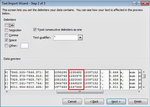
Select the "memory size after collection" field as shown above and compute the average as shown below:

Finally, the estimated live data size is 1359 MB.

Conclusions

If you have found that your live data set is large, you can improve your application's performance by:

• Reducing it by improving your codes
• For example, you should avoid object pooling which can lead both to more live data and to longer object life spans.
• Giving your application a larger heap
• As the complexity of a well written GC is mostly a function of the size of the live data set, and not the heap size, it is not too costly to support larger heaps for the same amount of live data. This has also the added benefit of it being harder to run into fragmentation issues and of course, implicitly, the possibility to store more live data.^[3]

Finally, what size of live data set is considered large. It actually depends on what GC collector you choose. For example, if you choose JRockit Real Time as your garbage collector, practically all standard application, with live data sets up to about 30 to 50 percent of the heap size, can be successfully handled by it with pause times shorter than, or equal to, the supported service level.^[3] However, if the live data size is larger than 50 percent, it could be considered too large.

References

1. JRockit: Out-of-the-Box Behavior of Four Generational GC's (Xml and More)
2. Back To Basics: Mark and Sweep Garbage Collection
3. Oracle JRockit- The Definitive Guide
4. JRockit: Parallel vs Concurrent Collectors (Xml and More)
5. JRockit: All Posts on "Xml and More"  (Xml and More)
6. JRockit R27.8.1 and R28.3.1 versioning 
• Note that R28 went from R28.2.9 to R28.3.1—these are just ordinary maintenance releases, not feature releases. There is zero significance to the jump in minor version number.

JRockit: Parallel vs Concurrent Collectors

The mark and sweep algorithm is the basis of all commercial garbage collectors in JVMs today.^[1,5,12] There are various implementations of mark and sweep algorithm in JRockit, which use different garbage collection strategies.

Unless you really know what you are doing, the –XgcPrio flag is the preferred way to tell JRockit what garbage collection strategies to run.^[1] However, if you want further control over GC behavior, a more fine grained garbage collection strategy can be set from the command line using the –Xgc flag.

In this article, we will examine four Generational Garbage Collectors (Generational GCs) in JRockit, which uses nursery.  Note that JRockit refers to the young generations^[2] as nurseries.

Generational Garbage Collection Strategies

The garbage collection strategy is defined by nursery, mark strategy and sweep strategy. The nursery  can either be present or not present. The mark and sweep phases can either be concurrent or parallel.

Here we only cover Generational GCs that use the nursery. For example, we will ignore "–Xgc:singlecon"—or single generational concurrent—in this discussion. As shown below, JRockit supports four different garbage collection strategies. They differ only in the using either concurrent or parallel in its mark and sweep phases.

-Xgc: option	Mark	Sweep
genconcon or gencon	Concurrent	Concurrent
genconpar	Concurrent	Parallel
genparpar or genpar (default)	Parallel	Parallel
genparcon	Parallel	Concurrent

GC Mode

Running JRockit with –Xverbose:gc will output plenty of verbose information on what the JVM memory management system is doing. This information includes garbage collections, where they take place (nurseries or old space), changes of GC strategy, and the time a particular garbage collection takes. For example, we have specified the following options:

-Xverbose:gc -Xverbosedecorations=level,module,timestamp,millis,pid

to find the GC mode of each strategy uses. As you can see, different strategies are designed for different purposes:

• Throughput, or
• Low lantency (or short pausetimes)

-Xgc: option	GC Mode
genconcon or gencon	Garbage collection optimized for short pausetimes, strategy: Generational Concurrent Mark & Sweep.
genconpar	Garbage collection optimized for short pausetimes, strategy: Generational Concurrent Mark, Parallel Sweep.
genparpar or genpar	Garbage collection optimized for throughput, strategy: Generational Parallel Mark & Sweep.
genparcon	Garbage collection optimized for short pausetimes, strategy: Generational Parallel Mark, Concurrent Sweep.

Stopping the World (STW)

Stopping the world means that collectors are halting all executing Java threads to run a collection cycle, thus guaranteeing that new objects are not allocated and objects do not suddenly become unreachable while the collector is running. This has the obvious disadvantage that the application can perform no useful work while a collection cycle is running.

Even though an algorithm such as mark and sweep may run mostly in parallel, it is still a complicated problem that references may change during actual garbage collections. If the Java application is allowed to run, executing arbitrary field assignments and move instructions at the same time as the garbage collector tries to clean up the heap, synchronization between the application and the garbage collector is needed. Stopping the world for short periods of time is necessary for most garbage collectors and this is one of the main sources of latency and non-determinism in a runtime.

Parallel vs Concurrent Collectors

The mark-and-sweep algorithm consists of two phases:^[5]

1. Mark phase
• In which, it finds and marks all accessible objects (or live objects).
• Marking is very parallelizable and large parts of a mark phase can also be run concurrently with executing Java code.
2. Sweep phase
• In which, it scans through the heap and reclaims all the unmarked objects.
• Sweeping and compaction (JRockit uses partial compaction to avoid fragmentation), however, tend to be more troublesome for parallelization, even though it is fairly simple to compact parts of the heap while others are swept, thus achieving better throughput.

Many stages of a mark and sweep garbage collection algorithm can be made to run concurrently with the executing Java application. Marking is the most critical of the stages, as it usually takes up around 90 percent of the total garbage collection time. The computational complexity of mark and sweep is both a function of the amount of live data on the heap (for mark) and the actual heap size (for sweep).

Parallel collectors require stop-the-world pause for the whole duration of major collection phases (mark or sweep), but employ all available cores to compress pause time. Parallel collectors usually have better throughput, but they are not a good fit for pause critical applications.

Concurrent collectors try to do most work concurrently (though they also do it in parallel on multi-core systems), stopping the application only for short duration. Note that the concurrent collection algorithm in JRockit is fairly different from both HotSpot's concurrent collectors (CMS^[3] and G1^[4] ).

Conclusions

In memory management, the time spent in GC is detrimental to an application's performance. So, minimizing the time spent in GC seems to be a good thing to achieve (or is it?). Collectors use simple stop-the-world strategy consumes less CPU time because it is simple and requires less bookkeeping. However, simple stop-the-world collectors halt all Java threads and they are not a good fit for pause critical applications.  Note that lantency is caused by not spending CPU cycle executing Java code.

Optimizing for low lantencies  is basically a matter of avoiding stopping the world and let the Java application run as much as possible. However, performing GC and executing Java code concurrently requires a lot more bookkeeping and thus, the total time spent in GC will be longer. Also, if the garbage collector gets too little total CPU time and it can't keep up with the allocation frequency, the heap will fill up and an OutOfMemoryError^[6-8] will be thrown by the JVM. Therefore, another key to low latency is to keep heap usage and fragmentation at a proper level.

To conclude, the tradeoff in memory management is between maximizing throughput and maintaining low latencies. In the real world, we can't achieve both at the same time.

References

1. Oracle JRockit- The Definitive Guide
2. Understanding Garbage Collection (HotSpot)
3. Understanding CMS GC Logs (HotSpot)
4. Garbage First Garbage Collector Tuning (HotSpot)
5. Mark-and-Sweep Garbage Collection
6. How to Debug Native OutOfMemory in JRockit (Xml and More)
7. Diagnosing OutOfMemoryError or Memory Leaks in JRockit (XML and More)
8. Diagnosing Java.lang.OutOfMemoryError (XML and More)
9. JRockit: All Posts on "Xml and More"
10. JRockit R27.8.1 and R28.3.1 versioning 
• Note that R28 went from R28.2.9 to R28.3.1—these are just ordinary maintenance releases, not feature releases. There is zero significance to the jump in minor version number.
11. JRockit: Out-of-the-Box Behavior of Four Generational GC's (Xml and More)